|
|
|
|
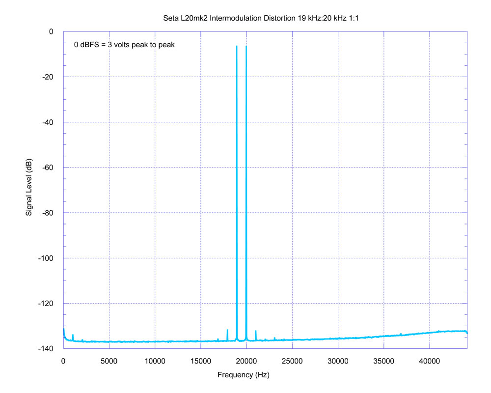
Seta L20 - Intermodulation Distortion (19 kHz : 20 kHz mixed 1 : 1) Measurement trap for young players: distortion is actually lower than it appears in the graph! Consider this: suppose we have an FFT trace such as shown above with baseline noise, and then inject a small bit of signal. Imagine that the baseline noise floor is a little lower than above (just to make this a little clearer - we'll examine this below in detail with "real" numbers), at -140 dB, and we inject a signal (say, a pure sine wave) with exactly a -134 dB level. Your first thought might be that you would see a signal bump in the FFT trace with a level of precisely -134 dB. However, that's not the case. The signal would add geometrically to the noise as the square root of the sum of the squares, and the peak would actually end up somewhat larger than -134 dB. The discrepancy will increase the closer the signal level gets to the noise floor (or, especially, a little bit below it)! Let's see how this happens. Stepping through the math Procedure: Convert the logarithmic decibels to linear (decimal) values, then square them, sum them, take the square root of the sum, then convert back to decibels. (Since this is a "gedanken" ("thought") experiment, and rather than get into a discussion about significant figures, we'll just retain all of the significant figures after the decimal point.) 1. Convert the logarithmic decibel values to linear (decimal) values. 10^(-140 dB / 20) = 0.000000100000000000000 10^(-134 dB / 20) = 0.000000199526231496888 (Note: The factor of 20 is used for decibel amplitude, expressed as a factor of volts below full scale. If we were calculating power, as in a power amplifier and using watts, a factor of 10 would be used because watts are the product of volts and amps, not just volts.) 2. Square the above values and add them together. (0.0000001 x 0.0000001) + (0.000000199526231496888 x 0.000000199526231496888) = 0.0000000000000498107170553497 Or made a little clearer with scientific notation: (1.0e-7 x 1.0e-7) + (1.199526231496888e-7 x 1.199526231496888e-7) = 1.0e-14 + 3.98107170553497e-14 = 4.98107170553497e-14 3. Take the square root of the result. √4.98107170553497e-14 = 2.23183146889163e-7 (or 0.000000223183146889163 as a decimal) 4. Convert to decibels. 20 x log10(2.23183146889163e-7) = -133.026772062913046 dB (The mathematically astute will recognize that we could have combined step 3 and 4, eliminating the square root calculation and using 10 instead of 20 as the multiplier.) Aha! That's a little bigger! Not -134 dB, but pretty close to -133 dB! If we repeat the above with a smaller sine, what happens? Let's try -146 dB. Skipping over the math, the result is (drum roll please): -139.026772062913046 dB. (Yes, the mantissa following the decimal point is the same as before.) So, even if a signal is "below" the noise floor (but not too far), it will still poke up above it. Here, by about a still-discernable 1 dB. Can we take a peak in the graph and then back-calculate what the true signal level is, as if there were no noise present? Sure we can. Just measure the level of the noise floor, square that, then measure the peak size, square that, subtract the noise floor then take the square root, and bingo. Using an example from the above graph, where the noise floor baseline is nice and flat (the numbers come from the data file from the measurement): 1. Noise floor baseline (from an average of several values adjacent to the peak) = -136.74 dB (again, averaged by first converting from decibels to decimal and then doing the math, and converting back to decibels; note that the average of -134 dB and -136 dB is not -135 dB; decibels are logarithmic, so adding logarithms is the same thing as multiplying the decimal values. Convert to decimal / linear representation first for addition / subtraction.) 2. The peak at 17 kHz: -135.87 dB After doing the above math, geometrically subtracting the baseline, we obtain the actual peak value of -143.28 dB. So, the amplitude is not -135.87 dB, but actually below the -136.74 dB noise floor at -143.28 dB: quite a bit lower! (You can verify this result by doing the calculation in reverse, using -136.74 dB and -143.28 dB; the resulting geometric sum is -135.87 dB.) The take-home message is that with signals close to the noise floor, one can't just take the value of the peak in the analyzer as the value of the signal! All of this actually can be verified experimentally, on the test bench. Just keep in mind that when working at the limits of the noise floor of a test and measurement setup, one may encounter issues with the nonlinearity of the ADC when resolving signals at the LSB level. (This isn't an issue for the DAC, since a high level signal would be generated then used with a precision attenuator in a test setup, to obtain the extremely low level test signals.) The solution is just to inject your own noise so the baseline is substantially above the noise floor, and work with larger signals. For example, with a very quiet measurement system (noise floor under -120 dB), mix in white noise to achieve a baseline noise level of, say, -90 dB and then experiment with injecting signals between -80 to -100 dB. Links to other Seta L20 measurements
|